Time-domain 특징
- Amplitude envelope (AE)
- Root-mean-square energy (RMS)
- Zero-crossing rate (ZCR)
Amplitude envelope (AE)
- 프레임 내 모든 샘플의 최대 진폭 값
- 음량에 대한 대략적인 정보 제공
- Outliers에 민감함
- Onset detection, 음악 장르 분류
Root-mean-square energy (RMS)
- 프레임에 있는 모든 표본의 RMS
- 음량 표시기
- AE보다 Outliers에 덜 민감함
- 오디오 세분화, 음악 장르 분류
Zero-crossing rate (ZCR)
- 타악기 소리와 음조 인식
- Monophonic pitch 단음 음조 추정
- 음성 신호에 대한 Voice/unvoiced 결정
1. Basic informations of audio files
Loading the libraries
1
2
3
4
5
import matplotlib.pyplot as plt
import numpy as np
import librosa
import librosa.display
import IPython.display as ipd
Loading audio files
1
2
3
debussy_file = "debussy.wav"
redhot_file = "redhot.wav"
duke_file = "duke.wav"
1
ipd.Audio(debussy_file)
1
ipd.Audio(redhot_file)
1
ipd.Audio(duke_file)
1
2
3
4
# load audio files with librosa
debussy, sr = librosa.load(debussy_file)
redhot, _ = librosa.load(redhot_file)
duke, _ = librosa.load(duke_file)
1
sr
1
22050
Basic information regarding audio files
1
debussy.shape
1
(661500,)
1
2
3
# duration in seconds of 1 sample
sample_duration = 1 / sr
print(f"One sample lasts for {sample_duration:6f} seconds")
1
One sample lasts for 0.000045 seconds
1
2
3
# total number of samples in audio file
tot_samples = len(debussy)
tot_samples
1
661500
1
2
3
# duration of debussy audio in seconds
duration = 1 / sr * tot_samples
print(f"The audio lasts for {duration} seconds")
1
The audio lasts for 30.0 seconds
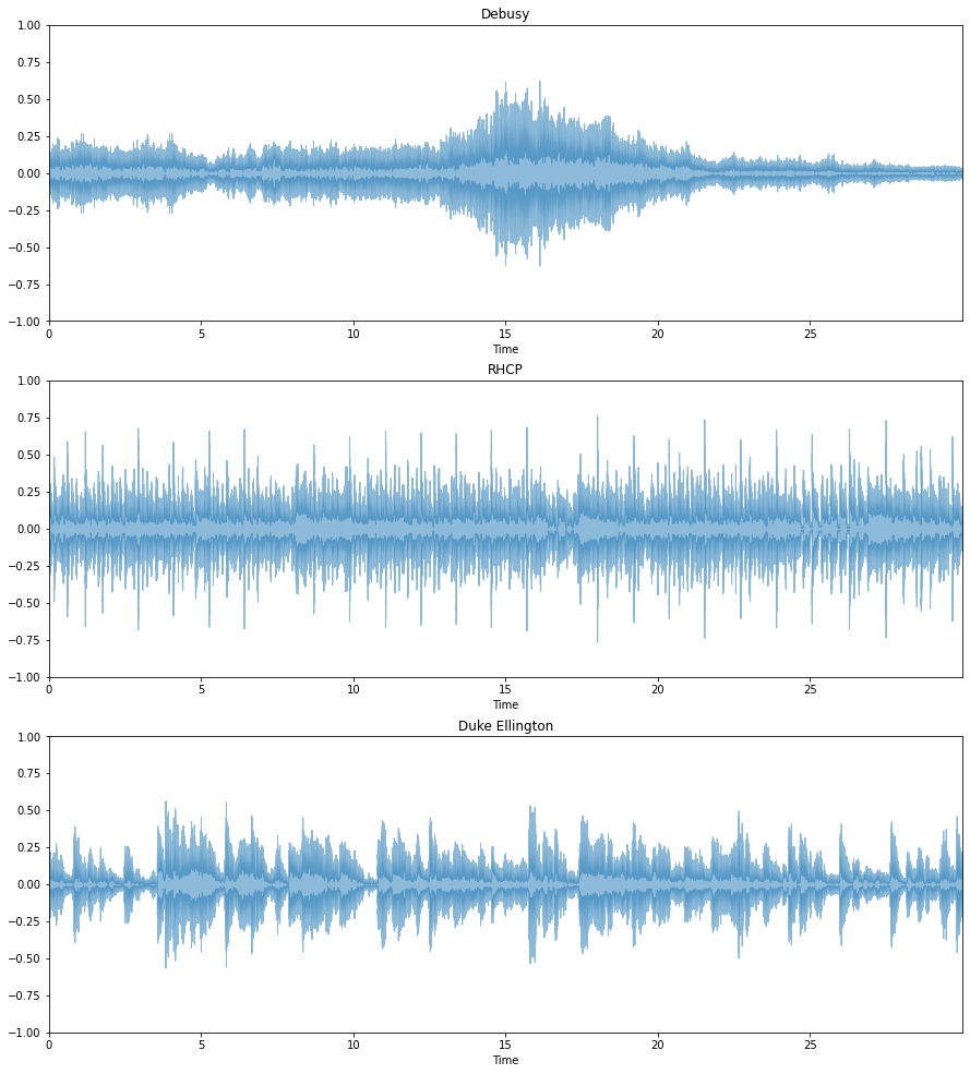
Visualising audio signal in the time domain
1
2
3
4
5
6
7
8
9
10
11
12
13
14
15
16
17
18
plt.figure(figsize=(15, 17))

plt.subplot(3, 1, 1)
librosa.display.waveplot(debussy, alpha=0.5)
plt.ylim((-1, 1))
plt.title("Debusy")

plt.subplot(3, 1, 2)
librosa.display.waveplot(redhot, alpha=0.5)
plt.ylim((-1, 1))
plt.title("RHCP")

plt.subplot(3, 1, 3)
librosa.display.waveplot(duke, alpha=0.5)
plt.ylim((-1, 1))
plt.title("Duke Ellington")

plt.show()
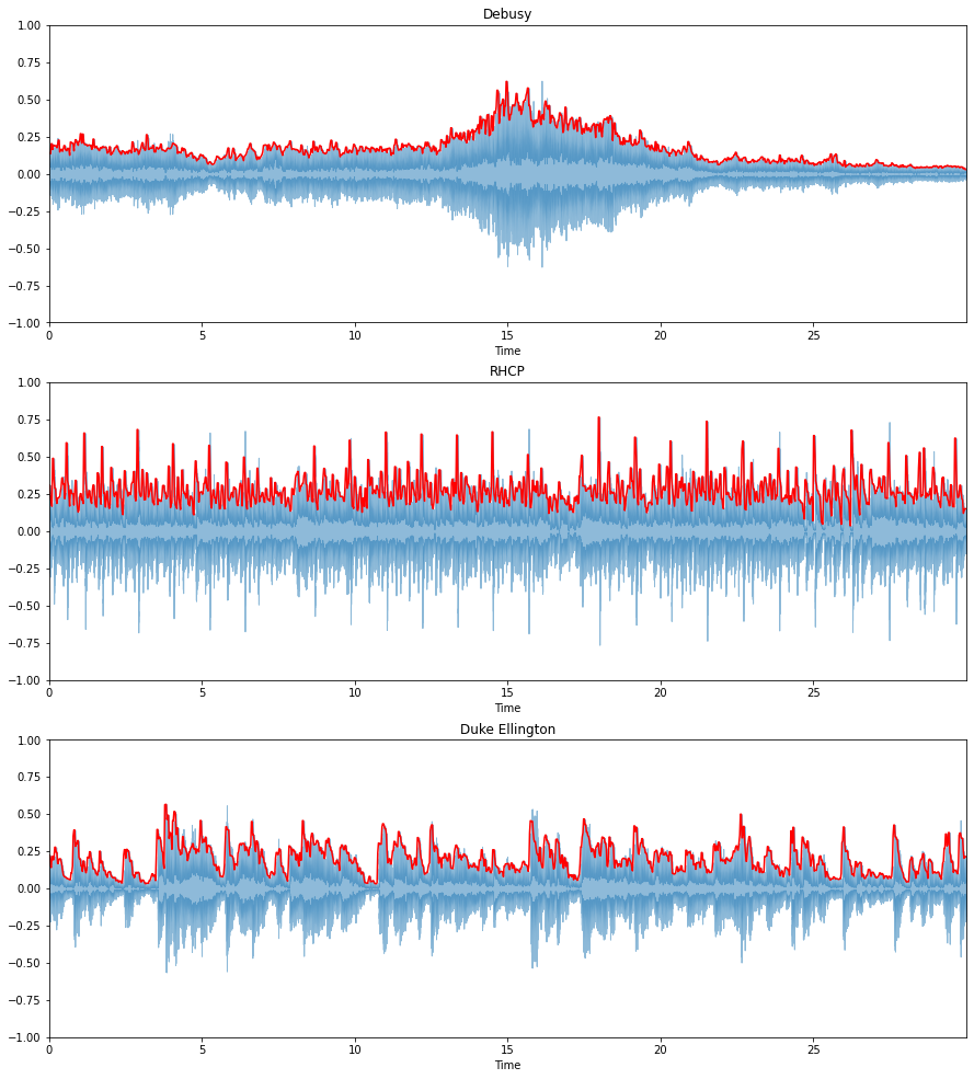
1. Extracting the amplitude envelope feature from scratch
Calculating amplitude envelope
1
2
3
4
5
6
7
8
9
10
11
12
13
FRAME_SIZE = 1024
HOP_LENGTH = 512

def amplitude_envelope(signal, frame_size, hop_length):
    """Calculate the amplitude envelope of a signal with a given frame size nad hop length."""
    amplitude_envelope = []

    # calculate amplitude envelope for each frame
    for i in range(0, len(signal), hop_length):
        amplitude_envelope_current_frame = max(signal[i:i+frame_size])
        amplitude_envelope.append(amplitude_envelope_current_frame)

    return np.array(amplitude_envelope)
1
2
3
def fancy_amplitude_envelope(signal, frame_size, hop_length):
    """Fancier Python code to calculate the amplitude envelope of a signal with a given frame size."""
    return np.array([max(signal[i:i+frame_size]) for i in range(0, len(signal), hop_length)])
1
2
3
# number of frames in amplitude envelope
ae_debussy = amplitude_envelope(debussy, FRAME_SIZE, HOP_LENGTH)
len(ae_debussy)
1
1292
1
2
3
# calculate amplitude envelope for RHCP and Duke Ellington
ae_redhot = amplitude_envelope(redhot, FRAME_SIZE, HOP_LENGTH)
ae_duke = amplitude_envelope(duke, FRAME_SIZE, HOP_LENGTH)
Visualising amplitude envelope
1
2
frames = range(len(ae_debussy))
t = librosa.frames_to_time(frames, hop_length=HOP_LENGTH)
1
2
3
4
5
6
7
8
9
10
11
12
13
14
15
16
17
18
19
20
21
22
23
# amplitude envelope is graphed in red

plt.figure(figsize=(15, 17))

ax = plt.subplot(3, 1, 1)
librosa.display.waveplot(debussy, alpha=0.5)
plt.plot(t, ae_debussy, color="r")
plt.ylim((-1, 1))
plt.title("Debusy")

plt.subplot(3, 1, 2)
librosa.display.waveplot(redhot, alpha=0.5)
plt.plot(t, ae_redhot, color="r")
plt.ylim((-1, 1))
plt.title("RHCP")

plt.subplot(3, 1, 3)
librosa.display.waveplot(duke, alpha=0.5)
plt.plot(t, ae_duke, color="r")
plt.ylim((-1, 1))
plt.title("Duke Ellington")

plt.show()
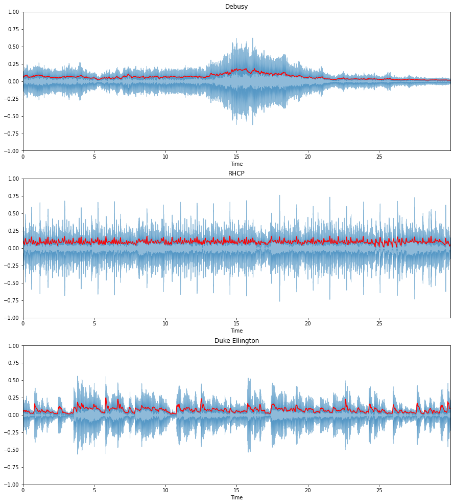
2. Extracting Root-Mean Square Energy
Root-mean-squared energy with Librosa
1
2
FRAME_SIZE = 1024
HOP_LENGTH = 512
1
2
3
rms_debussy = librosa.feature.rms(debussy, frame_length=FRAME_SIZE, hop_length=HOP_LENGTH)[0]
rms_redhot = librosa.feature.rms(redhot, frame_length=FRAME_SIZE, hop_length=HOP_LENGTH)[0]
rms_duke = librosa.feature.rms(duke, frame_length=FRAME_SIZE, hop_length=HOP_LENGTH)[0]
Visualise RMSE + waveform
1
2
frames = range(len(rms_debussy))
t = librosa.frames_to_time(frames, hop_length=HOP_LENGTH)
1
2
3
4
5
6
7
8
9
10
11
12
13
14
15
16
17
18
19
20
21
22
23
# rms energy is graphed in red

plt.figure(figsize=(15, 17))

ax = plt.subplot(3, 1, 1)
librosa.display.waveplot(debussy, alpha=0.5)
plt.plot(t, rms_debussy, color="r")
plt.ylim((-1, 1))
plt.title("Debusy")

plt.subplot(3, 1, 2)
librosa.display.waveplot(redhot, alpha=0.5)
plt.plot(t, rms_redhot, color="r")
plt.ylim((-1, 1))
plt.title("RHCP")

plt.subplot(3, 1, 3)
librosa.display.waveplot(duke, alpha=0.5)
plt.plot(t, rms_duke, color="r")
plt.ylim((-1, 1))
plt.title("Duke Ellington")

plt.show()
RMSE from scratch
1
2
3
4
5
6
7
8
def rmse(signal, frame_size, hop_length):
    rmse = []

    # calculate rmse for each frame
    for i in range(0, len(signal), hop_length):
        rmse_current_frame = np.sqrt(sum(signal[i:i+frame_size]**2) / frame_size)
        rmse.append(rmse_current_frame)
    return np.array(rmse)
1
2
3
rms_debussy1 = rmse(debussy, FRAME_SIZE, HOP_LENGTH)
rms_redhot1 = rmse(redhot, FRAME_SIZE, HOP_LENGTH)
rms_duke1 = rmse(duke, FRAME_SIZE, HOP_LENGTH)
1
2
3
4
5
6
7
8
9
10
11
12
13
14
15
16
17
18
19
20
21
22
23
24
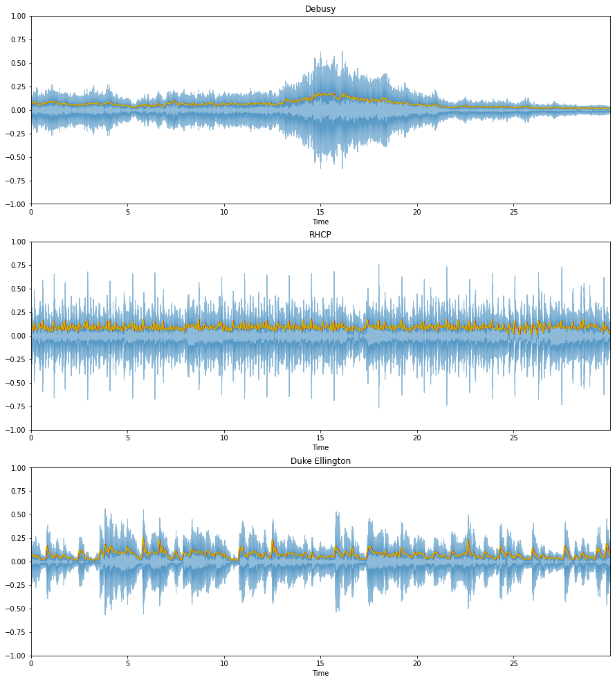
plt.figure(figsize=(15, 17))
ax = plt.subplot(3, 1, 1)
librosa.display.waveplot(debussy, alpha=0.5)
plt.plot(t, rms_debussy, color="r")
plt.plot(t, rms_debussy1, color="y")
plt.ylim((-1, 1))
plt.title("Debusy")
plt.subplot(3, 1, 2)
librosa.display.waveplot(redhot, alpha=0.5)
plt.plot(t, rms_redhot, color="r")
plt.plot(t, rms_redhot1, color="y")
plt.ylim((-1, 1))
plt.title("RHCP")
plt.subplot(3, 1, 3)
librosa.display.waveplot(duke, alpha=0.5)
plt.plot(t, rms_duke, color="r")
plt.plot(t, rms_duke1, color="y")
plt.ylim((-1, 1))
plt.title("Duke Ellington")
plt.show()
3. Extracting Zero-Crossing Rate from Audio
Zero-crossing rate with Librosa
1
2
3
zcr_debussy = librosa.feature.zero_crossing_rate(debussy, frame_length=FRAME_SIZE, hop_length=HOP_LENGTH)[0]
zcr_redhot = librosa.feature.zero_crossing_rate(redhot, frame_length=FRAME_SIZE, hop_length=HOP_LENGTH)[0]
zcr_duke = librosa.feature.zero_crossing_rate(duke, frame_length=FRAME_SIZE, hop_length=HOP_LENGTH)[0]
1
zcr_debussy.size
Visualise zero-crossing rate with Librosa
1
2
3
4
5
6
7
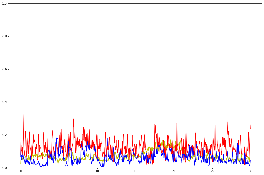
plt.figure(figsize=(15, 10))
plt.plot(t, zcr_debussy, color="y")
plt.plot(t, zcr_redhot, color="r")
plt.plot(t, zcr_duke, color="b")
plt.ylim(0, 1)
plt.show()
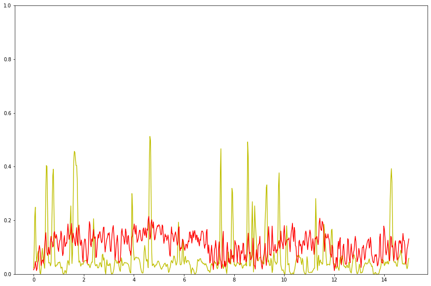
ZCR: Voice vs Noise
1
2
voice_file = "voice.wav"
noise_file = "noise.wav"
1
ipd.Audio(voice_file)
1
ipd.Audio(noise_file)
1
2
3
# load audio files
voice, _ = librosa.load(voice_file, duration=15)
noise, _ = librosa.load(noise_file, duration=15)
1
2
3
# get ZCR
zcr_voice = librosa.feature.zero_crossing_rate(voice, frame_length=FRAME_SIZE, hop_length=HOP_LENGTH)[0]
zcr_noise = librosa.feature.zero_crossing_rate(noise, frame_length=FRAME_SIZE, hop_length=HOP_LENGTH)[0]
1
2
frames = range(len(zcr_voice))
t = librosa.frames_to_time(frames, hop_length=HOP_LENGTH)
1
2
3
4
5
6
plt.figure(figsize=(15, 10))

plt.plot(t, zcr_voice, color="y")
plt.plot(t, zcr_noise, color="r")
plt.ylim(0, 1)
plt.show()